

 Product
 Brand
Brand Articles
 Tools
Tools
Norton's Theorem: Working Principle, Circuit Design, and Modern Applications
When analyzing complex electrical networks, calculating the voltage and current for a specific variable load can become a tedious process of repetitive mesh or nodal analysis. Norton's theorem provides a highly efficient shortcut. By condensing a complex network of power sources and resistors into a simplified model, engineers can rapidly evaluate how different loads will behave without recalculating the entire system.
In engineering exams and practical analysis, the application of norton's theorem to a circuit yields an equivalent current source and impedance in parallel. This fundamental principle—originally developed by Edward Lawry Norton at Bell Labs—remains a cornerstone of modern electronic design, bridging the gap between basic DC circuit theory and advanced power distribution network analysis.
The Core Principle of Norton's Theorem
Norton's theorem states that any linear one-port network containing independent voltage or current sources can be replaced by a single ideal current source (IN) in parallel with a single equivalent resistance (RN).
The primary advantage of this theorem is efficiency. When an engineer only needs to determine the current, voltage, or power of a single branch (the load), Norton's theorem isolates that branch. The internal network must be strictly linear (comprising standard passive components and linear power sources), but the external load circuit attached to the Norton equivalent can be non-linear. This makes the theorem exceptionally useful for testing variable loads, as the complex background circuit is reduced to just two constant values.
The 5-Step Workflow for Finding the Norton Equivalent Circuit
Deriving a Norton equivalent circuit requires a systematic approach. Expert demonstrations and visual circuit mapping highlight a strict five-step workflow to ensure accuracy:
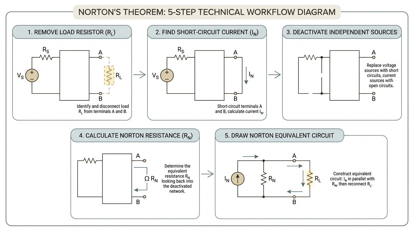
1. Remove the Load Resistor (RL)
The most frequent cause of failure in application is forgetting to isolate the load. The load resistor must be completely disconnected from the circuit, leaving two open terminals (often labeled A and B).
2. Calculate the Norton Current (IN)
Place a solid wire (a short circuit) across the open terminals A and B. The current flowing through this short circuit is the Norton Current (IN).
Expert Shortcut: In highly complex multi-branch circuits, calculating the short-circuit current directly can be messy. A proven engineering shortcut is to calculate the Thévenin open-circuit voltage (Vth) first using standard nodal analysis, and then derive the Norton current using Ohm's law: IN = Vth / RN.
3. Replace Independent Power Sources
To find the equivalent resistance, the circuit must be "deadened" by turning off all independent power sources. This follows the Ideal Source Replacement rule:
Independent Voltage Sources: Replaced by a short circuit (a solid wire, 0V).
Independent Current Sources: Replaced by an open circuit (a break in the wire, 0A).
Crucial Nuance: Dependent (controlled) sources must be retained. They cannot be zeroed out because their values depend on voltages or currents elsewhere in the circuit.
4. Calculate the Norton Resistance (RN)
With the independent sources zeroed and the load still removed, calculate the total equivalent resistance looking back into the circuit from terminals A and B. Visualizing the circuit is key here; for example, when a current source is opened, that specific branch is removed, which often turns previously complex parallel networks into simple series pairs.
5. Draw the Equivalent Circuit and Reattach the Load
Draw the final model: the current source (IN) in parallel with the resistor (RN). Finally, reattach the original load resistor (RL) across the terminals. You can now easily calculate the load current (IL) using the current divider rule.
📺 Norton's Theorem and Thevenin's Theorem - Electrical Circuit Analysis
Thévenin vs. Norton: Duality and Conversion
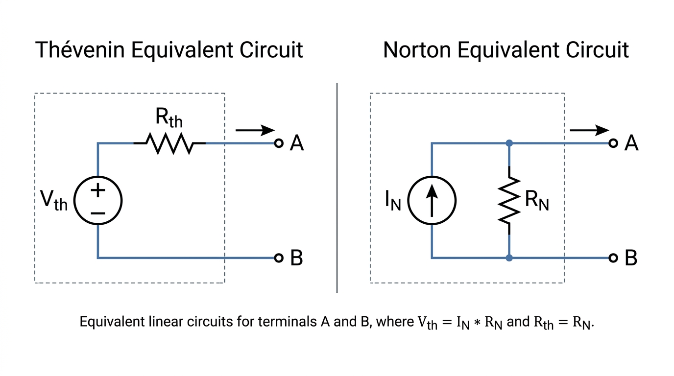
Norton's theorem is the exact mathematical dual of Thévenin's theorem. While Thévenin simplifies a circuit into a voltage source in series with a resistor, Norton simplifies it into a current source in parallel with a resistor.
Engineers often prefer Thévenin for voltage-driven analysis, but Norton is essential for current-focused scenarios. Because they are duals, you can easily convert between the two using Ohm's Law, provided the equivalent resistance (RN and Rth) remains identical.
| Feature | Thévenin Equivalent | Norton Equivalent |
|---|---|---|
| Equivalent Source | Voltage Source (Vth) | Current Source (IN) |
| Resistor Placement | In Series with the source | In Parallel with the source |
| Primary Use Case | Voltage-driven circuits, series load analysis | Current-driven circuits, parallel load analysis |
| Conversion Formula | Vth = IN × RN | IN = Vth / Rth |
| Equivalent Resistance | Rth | RN (Note: RN = Rth) |
Modern Engineering Applications
While textbook examples focus on simple DC resistor networks, Norton's theorem is heavily utilized in advanced modern engineering practices.
Power Distribution Networks (PDN) and High-Frequency PCBs
In high-frequency PCB design, ensuring stable power delivery to complex microchips is critical. When designing an Application-specific Integrated Circuit, engineers use Norton equivalents to model the Power Distribution Network (PDN). By simplifying the complex internal networks of the IC into a Norton equivalent, designers can accurately optimize the placement and values of decoupling capacitors to maintain power integrity.
EV Battery Management Systems (BMS)
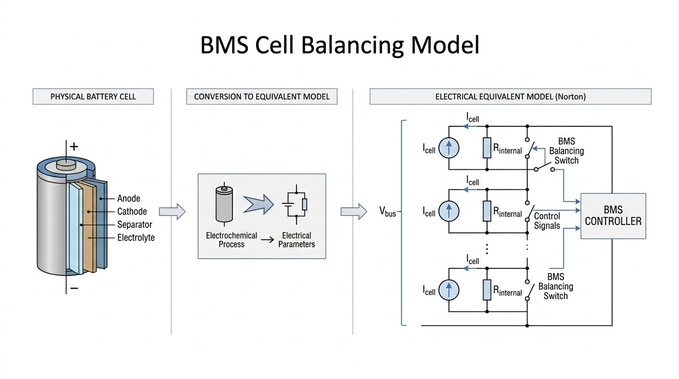
In electric vehicles, Battery Management Systems rely on Norton's theorem to evaluate short-circuit safety and develop battery equalization strategies. By modeling individual battery cells and their internal resistances as Norton equivalents, the BMS can calculate current distribution across multi-node distributed architectures, ensuring no single cell is overdrawn during rapid acceleration.
Current-Driven Optoelectronics
Norton's theorem is highly useful for analyzing current-dependent components. For example, when designing a driver for an RGB LED: Circuit, Difference and Application, engineers must manage precise current distribution across parallel lighting circuits. The Norton equivalent model allows designers to quickly calculate how current will divide among different LED branches without re-evaluating the primary power supply network.
Sensor Networks and Energy Harvesting
In IoT edge computing and sensor networks, the load resistance frequently changes based on environmental factors. By applying Norton's theorem, engineers can easily predict system behavior when swapping out a Commonly Used Sensitive Resistor Type Foundation and Circuit Application (such as a thermistor or photoresistor). The theorem is also used to model energy harvesting systems, like piezoelectric elements, which act as non-ideal current sources.
Fault Diagnosis and Sanity Checks
Norton's theorem provides a powerful framework for circuit troubleshooting and fault diagnosis. By establishing a baseline IN and RN for a healthy circuit, technicians can diagnose specific failures based on how the equivalent parameters change:
Increased RN: Typically indicates line aging, corroded contacts, or failing passive components.
Increased IN: Often points to a local short circuit bypassing intended resistive paths.
The "Sanity Check" Workflow:
Expert engineers never assume a manual Norton calculation is perfectly correct on the first try. A best practice is to perform a sanity check using KVL/KCL or SPICE simulations. By taking the final calculated load current and re-applying it back into the original complex circuit, you can verify if the resulting nodal voltages match the original power sources. If the ground reference potentials align, the Norton equivalent is verified.
What to Ignore in Circuit Simplification
When applying Norton's theorem, be aware of common pitfalls and outdated assumptions that can derail your analysis:
Ignore the "Target Resistor in Numerator" Myth: A frequent mistake when using the current divider formula to find load current (IL) is placing the load resistor in the numerator. The correct inverse logic dictates that the Norton Resistance must be in the numerator: IL = IN × [RN / (RN + RL)].
Ignore Circuits with Magnetic Coupling: Norton's theorem cannot be directly applied to circuits containing magnetic coupling (like transformers) unless the coupling is first resolved into an equivalent linear circuit model.
Do Not Ignore Initial Values: Norton calculations are highly sensitive to initial values. Misreading a single 5Ω resistor as an 8Ω resistor invalidates the entire RN and IN derivation. Always double-check component values before beginning the 5-step process.
Frequently Asked Questions (FAQs)
Q: Can Norton's theorem be applied to AC circuits?
A: Yes. While commonly taught using DC resistive circuits, Norton's theorem applies perfectly to AC circuits. The process is identical, but standard resistance (R) is replaced by complex impedance (Z), requiring phasor math to account for phase angles in capacitors and inductors.
Q: What happens if the circuit has no independent sources?
A: If a circuit only contains dependent sources and resistors, the Norton current (IN) will be zero. The circuit simply acts as an equivalent resistance (RN). To find RN in this scenario, you must apply an external test voltage or test current to the terminals and calculate the resulting response.
Q: Why must the internal network be linear if the load can be non-linear?
A: Norton's theorem is fundamentally based on the superposition principle, which only holds true for linear systems (where voltage and current scale proportionally). The internal network must be linear to be simplified. However, once simplified into a constant IN and RN, you can attach any non-linear load (like a diode) to the terminals and analyze it using load-line analysis.
Q: How does Norton's theorem help with maximum power transfer?
A: The Maximum Power Transfer theorem states that maximum power is delivered to a load when the load resistance equals the internal equivalent resistance of the source. By finding the Norton resistance (RN), you immediately know the exact value required for the load resistor (RL = RN) to achieve maximum power efficiency.
Q: Is it always better to use Norton over Thévenin?
A: Neither is universally better; it depends on the application. Norton is preferred when analyzing parallel circuits, current-driven components, or systems where nodal analysis is easier. Thévenin is generally preferred for series circuits and voltage-driven analysis. Because they are easily convertible, engineers often calculate whichever is mathematically simpler and convert to the other if needed.
 UTMEL
UTMEL
We are the professional distributor of electronic components, providing a large variety of products to save you a lot of time, effort, and cost with our efficient self-customized service. careful order preparation fast delivery service
 LLC Converter with Planar Matrix Transformer for High-Current-High-Power ApplicationsSaumitra Jagdale15 March 20245325
The rise of data centres in recent years, driven by cloud computing and big data, has caused a significant increase in electricity consumption. In the United States alone, it exceeded 70 billion kWh by 2014, making up 1.8% of total national electricity usage.
Read More Norton's Theorem: Working Principle, Circuit Design, and Modern ApplicationsUTMEL27 May 20261224
Norton's theorem simplifies complex linear electrical networks into an equivalent circuit containing a single current source in parallel with a resistor. This article explains the essential five-step workflow for calculating Norton parameters, compares it to its dual, Thévenin's theorem, and explores modern applications in power distribution networks, electric vehicle battery management, and fault diagnosis.
Read More SiC and GaN in 2026:How SiC and GaN Power Devices are Redefining AI Data Centers and 800V EVsUTMEL16 June 20263983
As AI data centers and 800V EVs hit physical thermal limits, the power electronics industry is shifting toward wide-bandgap semiconductors like SiC and GaN. This article explores how these materials are deployed in hybrid topologies to redefine power distribution, detailing high-voltage direct current architectures, engineering challenges in gate driving, and strategic sourcing solutions to build highly efficient, reliable modern power systems.
Read More Enhancing Frequency Stability in Modern Distributed Power SystemsRakesh Kumar, Ph.D.21 September 20244557
The article discusses the importance of primary frequency regulation in maintaining grid stability. It also explores battery energy storage systems, virtual synchronous generators, and advanced control strategies to enhance frequency stability in power systems.
Read More The Impact of SMPS on LED Lighting and Diverse IndustriesUTMEL05 June 20252881
Switched-Mode Power Supplies (SMPS) enhance LED lighting and industries by improving energy efficiency, reliability, and sustainability across diverse applications.
Read More
Subscribe to Utmel !
![HDC60D160H]() HDC60D160H
HDC60D160HSensata-Crydom
![JS1A-F-5V-F]() JS1A-F-5V-F
JS1A-F-5V-FPanasonic Electric Works
![2903702]() 2903702
2903702Phoenix Contact
![8881630000]() 8881630000
8881630000Weidmüller
![HDC60D120]() HDC60D120
HDC60D120Sensata-Crydom
![2903285]() 2903285
2903285Phoenix Contact
![LEV200AOANA]() LEV200AOANA
LEV200AOANATE Connectivity Aerospace, Defense and Marine
![2297057]() 2297057
2297057Phoenix Contact
![MY2K-US-DC12]() MY2K-US-DC12
MY2K-US-DC12Omron Automation and Safety
![AHES3292]() AHES3292
AHES3292Panasonic Electric Works


